1. Introduction
For variable climates, breeding is needed to identify genetic material that will function in the diverse environments where it will be cultivated. Both genetic diversity and the prediction of genotype responses to changes in environmental conditions are included in the problem. Structural variation offers a potential explanation for adaptive diversity, as pangenomic analysis of pearl millet has associated structural variants with heat tolerance, and extensive genomic variation has been associated with agronomic phenotypes from Setaria collected across locations and years [1], [2]. These resources provide an opportunity to assess if variants identified through graph representations are useful for ranking of breeding candidates in addition to conventional SNP predictors. Genomic selection relies on information from markers across the genome to predict quantitative performance without the need for each individual marker to be identified separately [3], [4].
It is dependent on the relationship between the population trained and that of the candidates being predicted. If genetic effects vary by environment, a model developed for average performance may not be as accurate for a specific target site. Reaction-norm models have been developed to account for this dependence and to represent the interaction between the genetic and the environmental factors [5], [6]. Thus, in addition to the information provided by the marker panel, environmental characterization provides information about how the genetic differences are expressed in different environments. Graph pangenomes solve another aspect of the prediction problem. The sequences and structural alleles that are exposed by multiple assemblies may represent only a partial view of the alleles contained in a single reference.
It is illustrative to look at comparative resources available in maize, wheat, barley, and rice, which reveal the level of diversity available via broader genomic representation [7], [8], [9], [10]. Such variation can be used computationally through graph-based mapping and genotyping of populations [11], [12], [13]. But better representation of improvement does not necessarily mean better prediction of improvement in all breeding populations. Other variants may overlap with already available SNP data and may offer different genomic coverage and/or genotype-call patterns that are associated with population structure. Environmental information also is of differing biological significance. Crop-stage exposures can differentiate stress during sensitive development stages while calendar summaries provide a more general description when planting and phenology records are unavailable.
Incorporation of environmental covariates has been found beneficial for improving prediction in studies on European maize, subtropical rice, and wheat production [14], [15], [16] and depends on the model and validation context. Evaluation design forms an integral part of the same dependence. Predicting a new accession at a previously observed location is a different effort from predicting a new accession in an entirely new environment. Differences between the two can be hidden by a single random partition and can be exaggerated when similar observations are split between training and testing sets [17]. The present study
integrates genetic and environmental information in a matched public-data experiment. Foxtail millet was chosen as it has an existing graph study, phenotype archive, and database with compatible accession identifiers and structural-variant calls [2], [18], [19]. The grain weight of the main panicle is analyzed in eight individually dated environments. Published SV calls are reused to determine their incremental contribution under explicit genetic and environmental transfer. The contribution is a controlled prediction comparison with ablations for alternative explanations for an increment; graph assembly and read processing are not part of the inherited resource. Climate-resilient breeding is the driving force behind the framework; the empirical end point is retrospective yield-component prediction across the observed network. Environmental interpretation is limited by realized calendar-year weather, incomplete management information, and the lack of available crop-stage dates. Hence, we analyze ranking information and its reliability—not correlative increases with proven tolerance or genetic gain.
1.1. Research questions
RQ1. To what extent do graph-derived SVs improve within-environment prediction and candidate ranking beyond a SNP reaction norm when locations, accessions, both factors, later years, or published population groups are held out? RQ2. Do SV-by-environment interactions contribute predictive information beyond SV main effects, and does their contribution depend on the transfer scenario? RQ3. How robust are apparent graph contributions to marker matching, SNP density, kernel rank, genotype coding, SV class, genomic proximity, and callability controls? RQ4. How do alternative environmental representations affect ranking and selection diagnostics, and what do the resulting differences imply for using this public resource in breeding-oriented prediction?
1.2. Research objectives
The overall goal is to evaluate the added value of the published graph-based variation in an environment-oriented cereal-prediction system. Specific goals are to: (i) build an auditable accession matched data set of phenotypes, SNPs, SVs, and weather; (ii) compare genetic main effects and reaction norms under five nested validation schemes; (iii) differentiate between added biological-variant information and model capacity, marker coverage, and marker call availability; and (iv) quantify ranking, prediction error, and top-set selection outcomes, and quantify the evidence for climate-resilience claims. These goals were not realized by using a primary configuration and substituting that configuration with another one that gave the highest possible
score in the sensitivity analysis, but by using a primary configuration and a list of sensitivity analyses that were declared.
2. Literature Review
2.1. Pangenomic diversity and graph-derived predictors
Cereal pangenomes demonstrate that there is a diversity of alleles beyond those contained in a single reference. The maize multi-assembly resource, the wheat genome comparison, and the barley pangenome all reveal variation that is relevant to breeding history or population diversity [7], [8], [9]. A rice super pangenome would take this one step further for differentiated rice lineages [10]. These studies justify broader genetic representation, but they are a resource and a biological-discovery study—and not a deployment study. A variant catalogue for genomic prediction should additionally be robustly associated with phenotyped accessions and assessed against an informative comparator. Graph-based tools are used for representing alternate sequences and their relationship in a reference structure.
The variation graph toolkit and further studies on structural-variant genotyping show how to interpret population reads against such representations [11], [12], [13]. Thus, a graph-derived predictor for a breeding analysis can be the output from an upstream graph-genotyping pipeline, while the downstream estimator is based on an accession-by-variant matrix. The difference lies here: the statistical model refers to the released structural allele categories and their relationships, and the construction of the graph and the processing of the reads are delegated to the source resource. In tomato, evidence suggests that a graph pangenome is able to model extra trait-associated variation and achieve better genetic analysis than a single-reference genome [20]. The pearl millet heat-tolerance study in cereals is a direct link between structural variation and an abiotic-stress phenotype [1].
The Setaria graph study combines population SV genotypes with extensive agronomic phenotyping and genomic-selection analyses [2]. More recently, graph pangenomics and association analysis and interpretable machine learning have been combined to prioritize presence-absence variants associated with pigmentation in Setaria [21]. These studies, combined, provide biological and computational motivations. Moreover, they emphasize that the combination of graph data and statistical learning is already a well-known research area.
2.2. Envirotyping and reaction-norm genomic prediction
Reaction-norm prediction is a prediction of the genetic performance that is conditional on the environment. This dependence can be modeled using a high-dimensional genomic and/or environmental covariance structure, which offers a practical way of modeling the dependence without estimating a separate effect for each marker–covariate combination [5]. The
marker-by-environment formulations in wheat are the same with regard to identifying stable genetic effects and environmental variable components [6]. The form of representation of the genetic and environmental effects has been reported to affect prediction in multi-environment trials by means of kernel extensions such as nonlinear relationships and dominance [22]. Such results encourage model comparisons and do not necessarily presume that the largest interaction model will be best. Envirotyping is the collection and re-expression of the environmental measurements to descriptors relevant for crop responses. EnvRtype is a software framework for linking environmental retrieval, ecophysiological processing, and quantitative-genetic analysis [23]. The importance of explicitly considering environmental conditions when making across-trial or across-year predictions is illustrated by applications in European maize and subtropical rice [14], [15].
This is further demonstrated by the environment-wide analysis of historical wheat data, which shows how environmental profiling can aid multi-year prediction [24]. These methods imply that environmental covariates may be useful, but determination of the proper temporal aggregation and biological alignment for a specific data set remain open questions. New research clarifies that question. The use of genotype-specific phenological environmental covariates has been introduced in the wheat random-regression models, and these crop exposure periods are more directly related to crop development [25]. Using envirotyping to predict the unobserved environments can be beneficial in a mega-environment dependent way for grain sorghum [26]. With wheat disease traits, comparisons between the environmental regression approach and the mixed-model approach show that improvement can vary with the nature of the relationship between training and target environments [27].
The present study employs calendar-month weather since the boundaries of the crop stages are not available in the public records selected. Alternative weather summaries are therefore considered substantive sensitivity analyses and not interchangeable preprocessing options.
2.3. Validation, model complexity, and breeding utility
As more genomic prediction algorithms are developed, more comparisons, with the same prediction task in mind, are necessary. Gradient boosting has been tested with maize traits, and reaction-norm analysis on Genomes to Fields data has been performed on both prediction and environmental variation of marker effects [28], [29]. An international genotype-by-environment prediction competition was recently held, which revealed several modelling strategies to provide useful estimates of maize yield [30]. Information on expected performance from algorithm labels is thus limited. Consideration of training information, target population, and environmental coverage/evaluation rules must be all taken together. Structured validation is one solution to this issue. Evaluation and transfer are more closely aligned if complete spatial, temporal, or hierarchical units are held out than if there is no restriction on record-level partitioning [17]. Another one that
separation of hyperparameter selection and final evaluation addresses is that the results of the
validation set may be used to select and evaluate the model, which can lead to optimistic estimates
[31]. These protections are also in effect for marker filtering, imputation, environmental scaling,
and learned feature representations in a multi-environment breeding dataset. When performed on
test accessions or test environments, those operations may change the apparent level of difficulty of
the operation even if test phenotypes are not included in the final regression. Prediction scores also
indicate various breeding utility components. Ordering or association is captured by correlations;
accuracy of the predicted trait scale is captured by absolute error; decisions close to a selection
threshold are captured by top-set metrics. An increase in one need not imply improvement in the
others. Prediction in multiple information scenarios is often done in a reaction-norm or
genomic-selection study [16], [6]. We extend this comparative logic to graph-derived predictors by
keeping common test candidates and looking at ranking, error, and selection as a whole. This
ensures that an improvement in mean correlation does not take the place of evidence of improved
breeding decisions universally.
2.4. Positioning the present contribution
Table 1 provides an overview of the studies that are most directly relevant to the empirical question.
The Setaria studies provide the source resource, the biological evidence from the pearl millet study
renders stress specific, and the environmental-prediction studies provide stress-relevant
response-modeling strategies. In the present analysis, we tackle this nexus between these lines of
research using a matched cereal cohort and a controlled comparison of the released SVs to a
reduced SNP baseline. The novelty is assessed at the empirical question and validation design level.
It is not reliant on the first use of pangenomes, machine learning, or reaction norms in the research
of crops.
Table 1. Selected primary studies and the position of the present comparison.
Study Relevant evidence Relationship to this analysis
Setaria graph resource [2]
Graph-derived SVs, agronomic phenotypes, and genomic selection
Inherited biological resource; the present study tests transfer and additional-channel controls.
Setaria graph and interpretable learning [21]
Pigmentation-associated PAV prioritization in 344 accessions
Here the endpoint is quantitative panicle-weight prediction across held-out settings.
Pearl millet heat tolerance [1]
Structural variation associated with a stress-specific phenotype
Provides biological motivation; calendar-weather grouping here is a coarser exposure definition.
Study Relevant evidence Relationship to this analysis
European maize prediction [14]
Environmental responses and phenological progression in yield prediction
Motivates explicit environment representation; crop-stage dates are unavailable here.
Phenology-informed wheat prediction [25]
Random regression with genotype-specific developmental covariates
Highlights the biological-resolution limit of calendar-month descriptors.
Sorghum envirotyping [26]
Prediction benefits depend on the mega-environment.
Supports testing context dependence across clearly defined transfer scenarios.
The specific question is, after taking into account marker count, missingness, capacity, and genomic
coverage, does an additional graph channel have predictive value in the context of genetic and
environmental transfers? Matched-marker and callability controls are used to control for
explanations that an unrestricted comparison does not take into account. Uncertain and negative
comparisons are kept, and graph main effects and environmental interactions are assessed
individually.
3. Methodology
3.1. Study design and public data sources
Secondary calculation was done for foxtail millet using publicly available genotype, phenotype
records, and meteorological records. The biological resource is based on the published Setaria
graph-pangenome study and the infrastructure of Setaria-db [2], [18]. Phenotypes were downloaded
from the Zenodo workbook Phenotypes_226.xlsx [19]. The accession identifiers in this workbook
are identical to those that are returned by the public Setaria-db genotype endpoint. No selection of
accessions for graph eligibility based on phenotype. The accession resource on Yugu1 v2.2 was
identified by the source database, and 680 accessions with the selected phenotypes and compatible
genotype were retained for analysis. The analytical sequence and the region between source
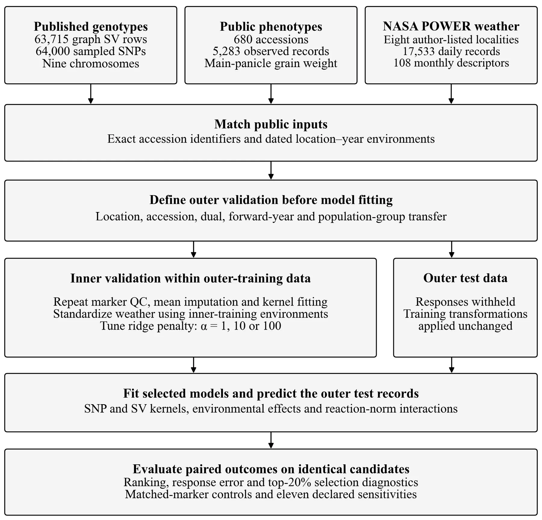
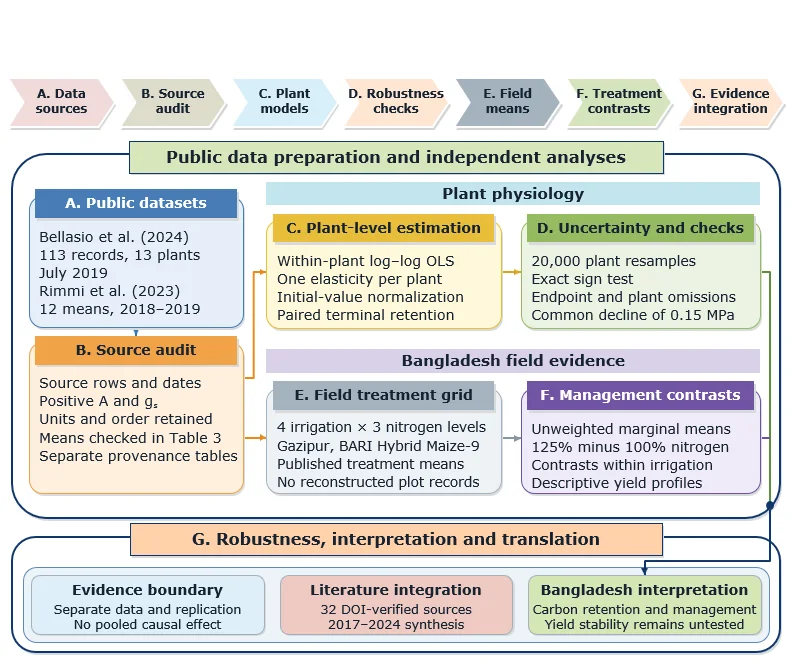
acquisition and model fitting are described in Figure 1. The genotype calls have been published and
were considered as an external fixed source. The common cohort was defined using phenotype
selection, dated-environment eligibility, and identifier matching prior to model comparison.
Training-dependent operations were then repeated for each validation split. This design was
selected because the SNP and graph comparisons could be interpreted on the same response records
and to maintain the computational feasibility of the analysis of the entire public data set. The graph
part was used: the use of the structural-variant calls that were published in the graph study; no graph
assembly or raw-read alignment was done.
No graph assembly or read alignment is needed—published calls are reused from the graph of Setaria. Geolocalization is available with the accession, which combines the genotype with the observed grain-weight records and with the locality coordinates (author listed). The outer splits are each followed by their own inner validation process, which involves redoing the genotype filtering, imputation, kernel estimation, and environmental scaling, and then selecting the ridge penalty. Responses from the outer test are not utilized in the fitting. The main group consists of eight environments, with the forward evaluation of five. The matched-marker controls are repeated in location and population transfer; all eleven sensitivity analyses apply the location-transfer setting.
3.2. Phenotype definition and environment eligibility
The response evaluated was the weight of the main panicle grain. This yield component was not independently verified from a released workbook to a physical unit, and the numbers were left in source trait units. We retained eight explicitly dated columns: Sanya 2010, Anyang 2011, Taiyuan
2013, Beijing 2016, Changzhi 2016, Urumqi 2016, Dingxi 2019, and Yulin 2020. Two pooled cross-year adjusted columns (Qitai and Qiqihar) were not included because it was not possible to determine a unique calendar year without using an unsupported temporal label. No missing phenotype was imputed, and missing response values were omitted. This resulted in 5283 accession-environment observations of 680 accessions. The retained environments, number of records, and annual weather descriptors are reported in Table 2. All 680 phenotypically identifiers were retained in both genetic matrices through exact accession matching. The genetic-structure labels were taken from Supplementary Table 1 of the source study: C1 (200 accessions), C2 (243 accessions), C3 (53 accessions), and Admixture (184 accessions) [2].
These labels were used to specify a population-transfer test. They did not count as pedigrees or proof of all the relatives being separated. Location holdout and environment holdout are the same in this data set, with each site holding for one year. Table 2. Retained phenotype environments and annual calendar-weather descriptors. Locality Year Records Mean trait Rainfall (mm) Hot days Sanya 2010 678 5.68 2282.4 0 Anyang 2011 679 8.16 615.0 45 Taiyuan 2013 674 10.27 549.1 0 Beijing 2016 670 9.49 681.1 12 Changzhi 2016 648 14.81 826.3 0 Urumqi 2016 667 20.82 352.7 18 Dingxi 2019 606 14.55 606.1 0 Yulin 2020 661 21.90 469.3 8
3.3. Genetic predictors and quality control
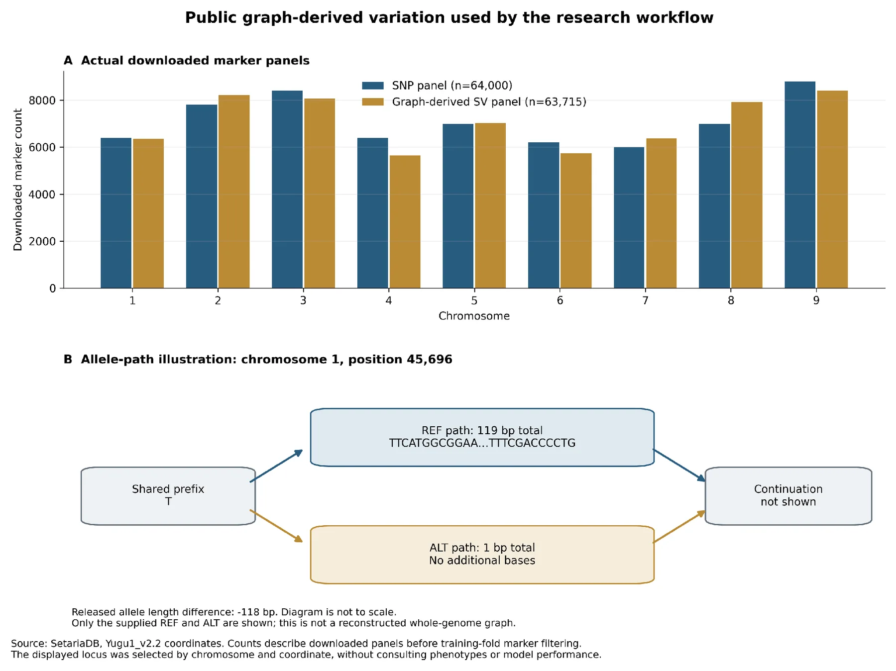
All nine chromosomes of the released (public) SV records for the matched accessions were retrieved from the public database export. The final input consisted of 63,715 rows of SVs. The set of 64,000 variants was chosen as 320 equally spaced blocks of 200 SNPs in a row from a provider's list of 4,934,313 variants arranged by chromosomal position. No phenotypes were used for the selection of these blocks. This downsized panel offered a manageable genome-spread coverage whilst still maintaining local clustering across blocks and only covered a proportion of the available SNP resource. To enable exact reconstruction of the retrieved release, source responses and request parameters and hashes of the files were preserved.
The chromosome-based inventory prior to the training-dependent filtering is provided in Figure 2A. The provider is shown in Figure 2B to have released its REF and ALT sequences at chromosome 1, position 45,696, which are 119 and 1 bp in length, respectively. This coordinate-selected example is not necessarily associated with any trait, nor is it necessarily a newly created graph or verified correspondence of the provider's plus/minus genotype category with REF/ALT orientation.
Figure 2. Downloaded genetic panels and a released structural-allele example. (A) Number of sampled SNPs and SV records (64,000 and 63,715, respectively) after each chromosome. (B) Provider's REF and ALT sequences at chromosome 1, position 45,696 on Yugu1 v2.2, are 119 and 1 bp in total length, respectively, for a released allele-length difference of −118 bp. The chromosome and coordinate of the locus were chosen based on no phenotypical information. It is a schematic graph of the alleles provided and is not to scale or of a complete genome [2], [18]. The SNP reference and alternate nucleotide calls were represented as 0 and 2. Minus and plus categories for the SVs were coded as "0" and "2" respectively without assuming their orientation to the reference and alternate sequences had been independently verified. Switching about the two categories at a locus reverses the sign of the centered values of that locus and does not affect the additive kernel contribution from that locus. For the conservative primary analysis, H and N were coded as missing. An explicit sensitivity that gives H a value of 1. A total of 13 complex SV
records were identified, which included undocumented nucleotide codes that were not able to be well-mapped to their long structural alleles; all calls at these records were masked in both encodings. Marker missingness and minor allele frequency were re-estimated within each training partition, based on the unique list of training accessions. Markers were excluded if the proportion of missing data was greater than 20% and/or if the minor allele frequency was less than 1%. Imputations were made for missing calls using the training-accession mean, and predictors were centered using the training estimates. Provenance was kept for provider-wide MAF and missingness rather than as model filters. These quantities were thus not constrained by the held-out accessions in the preprocessing. It did not negate any historical discovery and/or filtering that took place while the public resource was created. Dominance was not considered for the main inbred-panel analysis of SNP and SV channels, and the same rules and additive coding were used.
3.4. Environmental acquisition and envirotyping
The meteorological data were downloaded from the NASA POWER point API daily, with locality coordinates provided from the authors' source repository. Documentation of programmatic access to POWER is provided in the nasapower methods paper, and the meteorological products are based on the MERRA-2 atmospheric reanalysis [32], [33]. The public API was used directly on the Python workflow. Author-listed localities were used for coordinates; exact trial-plot GPS locations were not independently established. In each environment, the request included the calendar year that it was recorded in and the 5 previous calendar years. The complete retrieval contained 17,533 daily records. Before aggregation date continuity, duplicate dates, declared units, and physical bounds of humidity and precipitations were verified.
Twelve calendar months were the units of analysis, with nine different descriptors calculated: mean temperature, mean daily maximum temperature, mean daily minimum temperature, mean relative humidity, accumulated precipitation, mean daily surface shortwave radiation, approximate vapor-pressure deficit, number of days with maximum temperature above 35°C, and number of days with precipitations of 1 mm or more. This resulted in 108 environmental features. The vapor-pressure deficit was calculated daily from the daily mean temperature and relative humidity using the saturation-vapor-pressure relationship. Radiation was retained in MJ m⁻² day⁻¹ and precipitation in millimeters. The approximation is not able to recreate the demand of the atmosphere and the water deficit of crops on an hourly basis.
Three options were tried for environmental representation. Annual covariates were summed for rainfall, day counts, and averages by day for the rest of the descriptors. Each monthly feature was averaged over the previous 5 calendar years for a historical profile. A geographic control relied on only latitude and longitude. All environmental features have been centered and scaled, using different training environments. The primary models were the forecasts evaluated for retrospective transfer given the
realized weather in the target year. There were no verified planting dates, harvest dates, and irrigation management for alignment to crop stages. The historical profile limited its inputs to previous calendar years and did not appear as presowing forecasts for each of the trials. These choices are based on the general envirotyping philosophy of making explicit exposure definitions and testing their implications [23], [25].
3.5. Kernel construction and reaction-norm formulation
The combination of genetic main effects, environmental effects, and their interaction was done using low-rank multiple-kernel ridge regression. This formulation was selected for use because it can handle high-dimensional marker matrices via accession relationships, high-dimensional environment matrices, allow for prediction of unobserved accession–environment combinations, and allow for direct ablation of individual feature blocks. It is linked to kernel formulations for genomic selection and reaction-norm prediction [4], [5]. A fixed normalized block weights estimator was used with a chosen ridge penalty. It did not estimate separate genetic and environmental variance components using restricted maximum likelihood. For a training-centered marker matrix X, the linear genetic kernel was normalized by its mean diagonal. SNP and SV kernels were constructed separately using the same rule:
(1)𝐾 𝐺 = 𝑋𝑋 𝑇 𝑡𝑟(𝑋𝑋 𝑇 ) / 𝑛 𝐺 Here nG is the number of unique training accessions, and tr denotes the matrix trace. Missing-value imputation and centering occurred before kernel construction. Environmental relationships were obtained analogously from training-standardized environmental features. Positive-eigenvalue bases were retained with a maximum rank of 32 for each genetic channel and 6 for the environmental channel. Effective environmental rank was bounded by the number of training environments. A new accession was projected through its cross-kernel with the training accessions; it did not enter the eigenbasis fit. The rank-64 sensitivity assessed part of the approximation imposed by the primary genetic rank. If φS(g), φV(g), and φE(e) denote the fitted SNP, SV, and environmental feature vectors, interaction features were formed as tensor products: (2)ψ 𝑆𝐸 (𝑔, 𝑒) = φ 𝑆 (𝑔) ⊗ φ 𝐸 (𝑒), ψ 𝑉𝐸 (𝑔, 𝑒) = φ 𝑉 (𝑔) ⊗ φ 𝐸 (𝑒) Each included block was divided by its training root-mean squared row norm. This normalization placed channels on comparable training scales while leaving their relative weights fixed. The combined reaction norm can be expressed as:
(3)ŷ 𝑔𝑒 = μ + φ 𝑆 (𝑔) 𝑇 β 𝑆 + φ 𝑉 (𝑔) 𝑇 β 𝑉 + φ 𝐸 (𝑒) 𝑇 β 𝐸 + ψ 𝑆𝐸 (𝑔, 𝑒) 𝑇 β 𝑆𝐸 + ψ 𝑉𝐸 (𝑔, 𝑒) 𝑇 β 𝑉𝐸
The vectors β represent fitted coefficients for the corresponding feature blocks, and μ is an unpenalized intercept. Coefficients were obtained by minimizing the training sum of squared residuals plus a common ridge penalty over all included blocks:
(4)𝑚𝑖𝑛 μ,β ∑ (𝑔,𝑒)∈𝑇 (𝑦 𝑔𝑒 − ŷ 𝑔𝑒 ) 2 + α ∑ 𝑏∈𝐵 ‖β 𝑏 ‖ 2 , 𝐵 = {𝑆, 𝑉, 𝐸, 𝑆𝐸, 𝑉𝐸} The combination of genetic main effects, environmental effects, and their interaction was done using low-rank multiple-kernel ridge regression. This formulation was selected for use because it can handle high-dimensional marker matrices via accession relationships, high-dimensional environment matrices, allow for prediction of unobserved accession–environment combinations, and allow for direct ablation of individual feature blocks. It is linked to kernel formulations for genomic selection and reaction-norm prediction [4], [5]. A fixed normalized block weights estimator was used with a chosen ridge penalty. It did not estimate separate genetic and environmental variance components using restricted maximum likelihood. Table 3. Primary model specifications and their analytical roles. Model Included blocks Purpose
Environmental control E Environmental level; no within-environment ranking SNP main effects S Genetic-only reference SNP plus environment S + E No genomic interaction SNP reaction norm S + E + S×E Primary SNP comparator SNP reaction norm plus SV main S + E + S×E + V Separates SV main effects from SV interaction SNP plus SV reaction norm S + V + E + S×E + V×E Full primary model SV plus environment V + E Structural channel without SNPs SV reaction norm V + E + V×E Structural-only reaction norm S denotes SNP features, V graph-derived SV features and E environmental features. All models include an unpenalized intercept. Genetic kernels use maximum rank 32, environmental rank at most 6, and fixed training-normalized block weights. No dominance block is fitted.
3.6. Nested validation and prediction targets
There were five outer validation schemes, each unique in the use of the predictor. Locations were transferred with full sites. All records of selected accession identifiers were accession transferred. The accession set and the site set were both dual transfer, keeping the unseen accession–unseen site intersection as the test set and omitting the mixed quadrants. Earlier years were used to train the
forward validation, and then 2016, 2019, and 2020 were tested, respectively. Three grouped folds were used over the four published labels: one fold consisting of C2 and C3, and the other folds of C1 and Admixture. So the population test was not four leave-one-population-out fits but was a grouped transfer design. Each of the site, accession, and population schemes assessed 5283 records per model. Dual transfer tested 1,755 records, and transferred 3,252 records forward. The same held-out candidate sets and response values were employed in each model in a scenario. The forward evaluation was performed for five environments and the other schemes for eight environments. Given that the site was only found in one year, temporal transfer also meant moving the site.
The resulting scenarios are not interchangeable estimates from a common test population but can be compared as different information problems. Inner validation was performed in the same way as outer validation (up to three folds). The ridge penalty was chosen to be 1, 10, or 100 by mean within-environment Spearman correlation. The environmental-only control had an undefined ranking and thus a negative mean RMSE. Forward outer folds had one, two, and three admissible temporal inner folds, respectively, and population outer folds had two, three, and three inner folds. If structured folds were not available, no simpler random partition was used. Marker quality control, mean imputation, environmental scaling, kernel estimation, projection, and block normalization were performed on both inner and outer training sets.
This nesting is based on the protection measures against selection-induced optimism as per [31], [17].
3.7. Evaluation and paired uncertainty
Within-environment Spearman correlation between prediction and observed values of traits was the main metric. Pearson correlation, root-mean squared error, top-20% selection overlap, and selection regret were also calculated. First all the occurrences of an environment across accession or population folds were averaged. Reported aggregate scores then provided equal weight for environments, without an environment with more records dominating the summary. Between-environment differences can result in an association being spuriously high even if the ranking of accessions is weak, so no correlations were computed by aggregating all the sites into a single vector. For two models evaluated on the same candidates, the primary contrast was the difference between their mean environmental correlations:
(5)Δρ = 1 |𝐸| ∑ 𝑒∈𝐸 (ρ 𝑒
𝑆+𝑉 − ρ 𝑒
𝑆 ) During the uncertainty analysis, the site clusters were resampled with replacement while maintaining the combination of model scores. There were 2,000 draws for core and matched-marker comparisons and 1,000 draws for sensitivity comparisons. Descriptive 95 percent intervals were
given as the 2.5th and 97.5th percentiles. These intervals are based on the cross-validation results that have been fitted. They do not incorporate uncertainty from refitting all models, represent prediction intervals for individual accessions or measure transfer to an unspecified set of new populations. The number of sites are limited to 8, or five to forward transfer, so precision is limited. No multiplicity adjusted confirmatory test was performed, intervals were descriptive with several comparisons. The use of a conditional interval to exclude zero was not used independently to claim statistical significance for any broad claim. The ceiling of 0.2n was k, for n test candidates in the environment. Selection overlap was the percentage of the observed top-k set that was also in the model-selected top-k set. Selection regret was defined as the difference between the traits observed in those two selections:
(6)𝑅 𝑒 = 1 𝑘 ∑ 𝑔∈𝑂𝑒 𝑦 𝑔𝑒 − 1 𝑘 ∑ 𝑔∈𝑃𝑒 𝑦 𝑔𝑒 , 𝑘 = ⌈0. 2𝑛 𝑒 ⌉ Lower regret indicates a selection closer to the observed within-test optimum. It remains an evaluation statistic in source trait units, not a measured response to a breeding cycle. A deterministic accession-identifier tie break was used when predictions tied. Environmental-only selection statistics therefore describe that arbitrary tie break and were excluded from substantive claims about ranking ability.
3.8. Matched-marker controls and sensitivity analyses
Matched-channel comparisons for location and population transfer were performed. For each training fold, up to 1024 SV–SNP pairs were chosen that were close according to the following criteria: minor allele frequency, missingness, equal number of markers, additive coding, and highest spectral rank. Matching allowed for a maximum difference of 0.05 for both missingness and minor allele frequency and no use of the same marker within a match. The baseline SNP reaction norm was compared to a matched SNP channel, matched SV main effects, and matched SV main plus interaction effects. Within the nested procedure, matching was done with used training accessions and repeated. The added SNP channel was used as a control channel because it was identical to the initial channel and contained the same markers already represented in the baseline channel.
It did not add a new and independent SNP panel. Matching did not equalize the linkage disequilibrium or depth of sequencing or functional annotation. The cohort and splits used in each of the 11 prespecified sensitivities were the same as those used in the location-transfer cohort. They assessed annual weather, weather over the previous 5 years (moving window), geography alone, 16,000 SNPs, 32,000 SNPs, genetic rank 64, H encoded as 1, simple insertion SVs, simple deletion SVs, SVs within 50 kilobases (kb) of a sampled SNP, and SV callability indicators. The original block-sampling design was maintained for the smaller SNP
panel. The simple class was not assigned to ambiguous sequences but was determined from explicit reference and alternate sequences after trimming away shared anchors for pure insertions and deletions. The proximity restriction was not a linkage-disequilibrium match but a genomic-coverage sensitivity. Callability employed called-versus-missing indicators instead of biological allele categories, and these were interpreted separately. Held-out predictions were also broken down by calendar-weather conditions. Without considering their phenotypes, high-heat and low-rainfall thresholds were established from outer-training environments, and test environments were assigned. These groups were descriptive exposure categories. Annual rainfall amounts were not considered as evidence of a drought treatment—also because irrigation was not completely documented. Held-out location predictions were summarized as mean and lower quartiles of predicted percentiles within environments. The candidate table offers a description of the ranking based on the observations of the entire network and does not attempt to make any claims to realized gain or future-climate robustness.
4. Results
4.1. Cohort coverage and environmental contrast
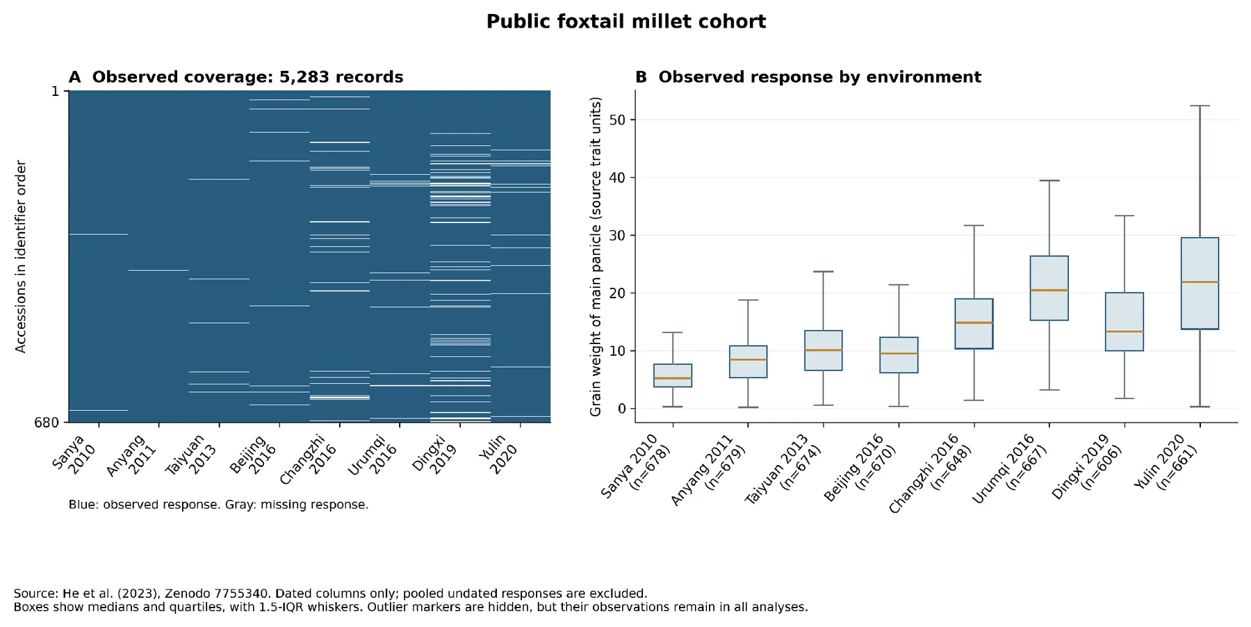
The 680 phenotype accessions all matched both genetic data sources, leaving a common set of accessions for the SNP and graph comparisons. The number of possible combinations of accession and environment, 5,440, was achieved to 97.1% (5,283 combinations). Counted numbers varied from 606 at Dingxi to 679 at Anyang. As observed from the response distribution as well as the environmental descriptors in Table 2, there was a variance of response in the network. The mean panicle grain weight varied from 5.68 source units at Sanya to 21.90 at Yulin. Such differences indicate the need to distinguish the effects of environmental trait levels from within environment accession ranking but do not, in themselves, represent a weather effect, as sites had different years and unmeasured conditions. The near-complete observed coverage is shown in Figure 3A, where there are also some gaps in the observations that are not uniform across environments. The individual response distributions are shown in source trait units in figure 3B. For ease of viewing, outlier symbols are omitted from the boxplots, but all of the records observed are kept in the analysis.
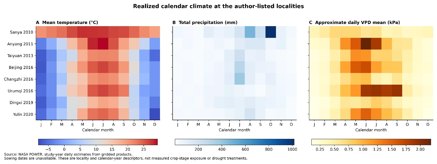
Figure 3. Observed phenotype coverage and response distributions. Accessions are sorted by identifier, and (A) blue cells indicate observed grain-weight records and grey cells indicate missing responses in 680 accessions in 8 dated environments. There are 5283 observed records in the cohort. (B) Boxplots display the response distribution in source trait units and the number of samples for each environment. Boxes extend across the interquartile range with the central line indicating the medians, and whiskers indicate the observations that are within 1.5 interquartile ranges. Outlier symbols are not shown, but the outlier observations are included in the analysis. No imputations were made for missing responses [2], [19]. The monthly mean temperature, accumulated precipitation, and approximate vapor-pressure deficit are shown in panels A, B, and C of Figure 4, respectively.
The tropical locality of Sanya is compared to the northern localities with high seasonal changes based on temperature profiles, and descriptions of environmental heterogeneities are also included based on precipitation and vapor-pressure deficit. The annual rainfall varied from 352.71 mm at Urumqi to 2,282.39 mm at Sanya. Days with a maximum temperature above 35°C were counted at each site-year and were 45 days at Anyang, 18 days at Urumqi, 12 days at Beijing, 8 days at Yulin, and 0 days at the other site-years retained. These are calendar-weather terms that are attached to a grid. They offer environmental contrast but not crop-stage heat exposure or water limitation.
Figure 4. Realized calendar-month weather at the author-listed localities. The panels show monthly mean temperature (A), accumulated precipitation (B), and the monthly mean of approximate daily vapor-pressure deficit (C). Values are based on the NASA POWER estimates for each site-year, and the month labels are January, February, etc. Vapor-pressure deficit was estimated using mean daily temperature and relative humidity. These are locality-level calendar descriptors. They are not necessarily indicative of the weather conditions at recognized crop-development stages, field water deficits, or drought conditions under experimentation [32], [33]. The primary genotype encoding yielded missing fractions of 4.64% for SNPs and 9.59% for SVs. Before training filtering, one SNP and 44 SV rows were entirely missing, including the 13 deliberately masked ambiguous SV records. In the site-holdout fits, all 680 accession identities remained represented in training through their other environments, and quality control retained 33,078 SNPs and 34,429 SVs. The rank-32 bases captured approximately 50.9% of the positive SNP-kernel trace and 38.1% of the SV-kernel trace in these fits. Thus, the nominal downloaded marker counts and the effective fitted representations are distinct. The lower SV trace retention also provides a concrete reason to inspect the rank sensitivity.
4.2. Primary prediction across transfer scenarios
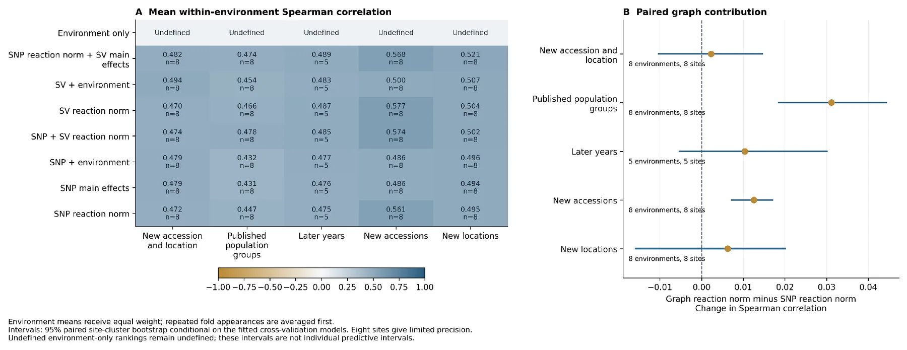
Means of the Spearman correlations for all eight primary models are reported within environments in Table 4. The combined SNP–SV reaction norm was greater than the SNP reaction norm in both scenarios, but the differences were small compared to the differences between the prediction tasks. Correlations for predicting new-accession were 0.5612 for the SNP reaction norm and 0.5737 for the combined model. Population transfer resulted in 0.4468 and 0.4780, respectively. Location transfer yielded 0.4953 and 0.5016; dual transfer yielded 0.4721 and 0.4744; and forward transfer yielded 0.4750 and 0.4854. The answer to RQ1 is provided by these results, as both the evaluated configurations resulted in a positive mean increment, with significant variations in its value and accuracy.
Table 4. Mean within-environment Spearman correlation across the eight primary models.
Model New locations
New accessions
Dual transfer Later years Population groups
Environmental control — — — — —
SNP main effects 0.4943 0.4862 0.4789 0.4762 0.4307
SNP plus environment 0.4963 0.4856 0.4794 0.4770 0.4319
SNP reaction norm 0.4953 0.5612 0.4721 0.4750 0.4468
SNP reaction norm plus SV main 0.5207 0.5680 0.4821 0.4893 0.4745
SNP plus SV reaction norm 0.5016 0.5737 0.4744 0.4854 0.4780
SV plus environment 0.5066 0.4998 0.4941 0.4831 0.4541
SV reaction norm 0.5041 0.5767 0.4695 0.4868 0.4660
Each environment receives equal weight after repeated fold appearances are averaged. Dual transfer
tests new accessions at new sites. Population groups are published structure labels. An em dash
denotes an undefined correlation for the environmental-only control. Five environments contribute
to forward evaluation, and eight to each other's scenario. Paired uncertainty is shown in Figure 5B.
Figure 5. Primary model comparison and paired contribution of the combined SNP–SV reaction norm.
(A) Mean within-environment Spearman correlation for eight models; n is number of contributing environments, not accessions or validation folds. When folded multiple times, appearances in the same environment are averaged; then, environments are weighted equally. Within-environment predictions are constant, and environment-only correlations are undefined. (B) Points show the combined SNP–SV reaction norm minus the SNP reaction norm; horizontal lines are conditional descriptive 95% percentile intervals from 2,000 paired site-bootstrap draws. There are 8 sites in each comparison (5 in later-year transfer). The plotted graph reaction norm is the combined SNP–SV model. The intervals are merely for the fitted models and are not individual predictive uncertainty. The combined-versus-SNP reaction-norm differences are presented on a paired scale (Figure 5B) and are compared to all eight primary models (Figure 5A).
The largest increase was 0.0311 for population transfer with a conditional descriptive interval of 0.0185 to 0.0443. The new-accession increment was 0.0126, with an interval of 0.0072 to 0.0170. Location transfer had an increment of 0.0063 and an interval of −0.0158 to 0.0200. Dual and forward increments were 0.0023 and 0.0104, with intervals of −0.0103 to 0.0145 and −0.0053 to 0.0300. The last three intervals include contributions that are not statistically significant but also changes in both directions. The population and accession intervals are a measure of stability across the site scores observed conditional on the fitted models and not a measure of equivalent precision in new genetic groups or a new trial network.
4.3. Interaction ablation and competing model explanations
Not all of the combined reaction norm models were the top models in each situation. However, the SNP reaction norm (with SV main effects) was found to be 0.5207 for location transfer, which is higher than the full interaction model (Table 4). New-accession prediction was slightly better, with an SV-only reaction norm of 0.5767. The SV-plus-environment model was able to account for the dual transfer at a higher value of 0.4941 than the combined reaction norm (0.4744). These other options show that, for some targets, the most sophisticated channel and interaction mix is not necessary and may not be as effective, yet the graph source can still have valuable relationship information. The interaction ablation compares the full model to the SNP reaction norm model plus SV main effects (Table 4, Figure 5A). The complete model modifications Spearman correlation by −0.0191, −0.0077, and −0.0039 for location transfer, dual transfer, and forward transfer, respectively, when compared to this ablation. The accession and population transfers were +0.0057 and +0.0035, respectively. Thus, the answer to RQ2 is transfer dependent. The results advocate the distinction of the main effect of the graph from the interaction of the graph as opposed to one
inseparable source of benefit. They also warn that gains compared to SNP baseline should not be attributed to the environmental modulation of SV effects.
4.4. Absolute prediction and selection outcomes
Absolute error and selection diagnostics of the SNP and combined reaction norms are compared in table 5. The mean RMSE was reduced from 5.0212 to 4.9501 source units for accession transfer and from 5.3674 to 5.2574 source units for population transfer. It also decreased slightly in dual transfer, from 6.6634 to 6.6446. However, for location transfer the RMSE rose from 6.7509 to 6.7897, and for forward transfer it rose from 8.8482 to 8.9169. The prediction of the magnitude of the trait from a good ranking increment was not consistent, however. The relatively high forward errors are consistent with a challenging temporal/geographical transfer task but may not be attributed to climate extrapolation alone. Table 5. Absolute prediction error and retrospective selection outcomes. Validation RMSE Selection regret Top-set overlap (%) New locations 6.751 → 6.790 5.253 → 5.036 36.08 → 37.62 New accessions 5.021 → 4.950 4.534 → 4.376 42.84 → 44.03 New accessions and locations 6.663 → 6.645 4.901 → 4.822 39.21 → 38.89
Later years 8.848 → 8.917 6.357 → 6.101 36.19 → 37.14 Population groups 5.367 → 5.257 5.200 → 5.153 36.42 → 36.68 Each cell reports the SNP reaction norm → SNP plus the SV reaction norm. Lower RMSE and regret are preferable; higher overlap is preferable. RMSE and regret retain source trait units. Selection uses the best predicted 20% of test candidates, rounded upward. Values are equal-environment means, with repeated test appearances averaged first. In all five comparisons the mean selection regret decreased, with the greatest absolute decrease in forward transfer (6.3571 to 6.1014 source units). Location-transfer regret decreased from 5.2535 to 5.0357, and accession-transfer regret from 4.5338 to 4.3758.
Top-set overlap is also shown in Table 5. There was an increase in overlap of around 1.54 percentage points for locations, 1.19 for accessions, 0.95 for later years, and 0.26 for population groups. It decreased by around 0.31 percentage points in the dual transfer. As seen in that case, there can be a difference between overlap and regret and still be a similar or slightly better observed mean trait value when choosing a set with a smaller number of identical members. These diagnostics link prediction with selection on the candidate sets that are also held out. A decrease in regret is an after-the-fact outcome but has not been quantified in terms of a response in the breeding cycle.
Since substantive interpretation cannot
be made by the environmental-only selection outcome, this was not included. Candidate stability rankings also refer to predicted percentiles across the observed network.
4.5. Matched-marker and extra-channel controls
The matched comparisons for location and population transfer are provided in Table 6. The baseline correlation for the SNP in the location analysis was 0.4953. Matched SV reaction-norm channel addition resulted in 0.4973, an increase of 0.0021, but with a conditional interval of −0.0219 to 0.0168. The sum of the matched SV main effects was 0.5158. The additional matched SNP channel resulted in 0.4835. This gave the matched SV interaction model a 0.0138 points advantage over the extra SNP-channel control but a negligible and questionable advantage over the plain SNP baseline. This is important because the additional SNP channel reused markers and could change regularization without providing new genetic information.
Population transfer kept a lower matched graph increment. The baseline score was 0.4468, while that for the matched SV reaction norm was 0.4554, with an interval of 0.0007 to 0.0157. The matched SV main effects produced 0.4531, while the additional matched SNP channel produced 0.4456. The gap between the matched and unrestricted graph increments agrees with the overall panel and representation impact on the unrestricted graph. Matching alters the number and kinds of predictors, and therefore does not uniquely diagnose the source of that change. It does demonstrate that the larger unrestricted population increment is not necessarily an effect of feature-panel design. Table 6. Matched-marker comparisons in location and population transfer.
Model New locations Population groups SNP reaction norm 0.4953 0.4468 SNP reaction norm plus matched SNP channel 0.4835 0.4456 SNP reaction norm plus matched SV main 0.5158 0.4531 SNP reaction norm plus matched SV reaction norm 0.4973 0.4554 Training-fold matching retained 1,024 SNP–SV pairs with maximum MAF and missingness differences of 0.05. The extra SNP channel reuses baseline SNPs. Matched SV reaction-norm increments over the SNP baseline were 0.0021 (−0.0219 to 0.0168) for locations and 0.0086 (0.0007 to 0.0157) for populations; intervals are conditional descriptive 95% site-bootstrap intervals.
4.6. Environmental, genomic, and callability sensitivities
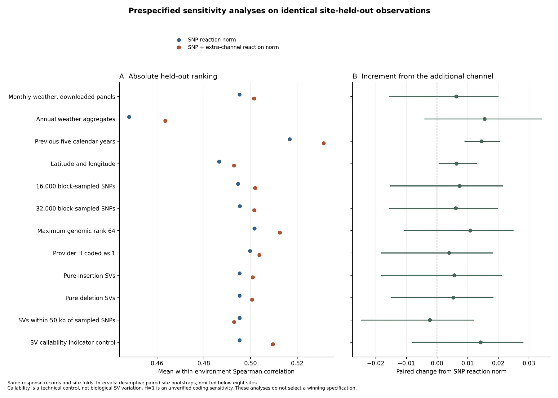
All 11 sensitivity analyses performed using the common location-transfer design. Absolute ranking correlations are shown in Figure 6A, and paired additional-channel increments are shown in Figure 6B for the primary analysis and sensitivities. The preceding-five-calendar-year profile yielded correlations of 0.5168 for SNPs and 0.5313 for SNPs plus SVs, versus 0.4953 and 0.5016 in the main profile. It had a graph increment of 0.0145 and a conditional interval of 0.0091 to 0.0203. The absolute correlations for annual weather and geographic control were 0.4480 and 0.4635, respectively. These differences provide a response to RQ4: differences in the baseline as well as the apparent graph contribution due to environmental representation. Inspecting performance should be done in conjunction with the historical-profile gain, not as an alternative to the primary specification, which has a higher absolute RMSE.
Reducing the SNP panel to 16,000 or 32,000 markers yielded graph increments of 0.0073 and 0.0062, close to the primary 0.0063. This stability is in the context of the stated block-sampling design. Absolute correlations increased with the higher genetic rank (up to 64), to 0.5017 (SNPs) or 0.5126 (combined model); however, the 0.0109 increment remained above zero. Coding H as 1 produced correlations of 0.4998 and 0.5038, with an increment of 0.0040. The small positive increments of approximately 0.0056 and 0.0053 were also observed for pure insertion and deletion channels, respectively, with intervals that intersect the zero value. No single class of SV or coding alternative can be identified from these results that provides a clear location-transfer advantage.
Figure 6. Absolute ranking and additional-channel effects in the location-transfer sensitivity analyses. The primary monthly-weather comparison and eleven sensitivities are made using twelve rows of identical held-out response records and site folds. (A) Points show mean within-environment Spearman correlation between the SNP reaction norm and the model with the added channel. Points indicate their paired difference; horizontal lines are conditional descriptive 95% percentile intervals from 1000 site-bootstrap draws. There are 8 environments and 8 sites per row. The callability row does not change SV allele categories to called-versus-missing indicators and is a technical control; H coded as 1 is still an unverified encoding sensitivity. The interval for the primary row is slightly different from that in Figure 5B since the number of bootstrap draws is different.
Two controls proved to be especially helpful for RQ3. Filtering the graph channel to only the 6,436 SVs within 50k of sampled SNPs gave a correlation of 0.4930, whereas the SNP baseline had a correlation of 0.4953. The increment was −0.0023, with an interval of −0.0246 to 0.0119. This restriction alters the number of markers counted, the composition of markers, and the coverage and therefore is not a pure causal test of genomic location. Still, it indicates a lack of persistence in the small unrestricted gain for this restricted panel. The comparison also suggests the reasons for a dense SNP baseline and explicit linkage-disequilibrium matching would be valuable in a larger replication.
The callability-control reaction norm resulted in a higher correlation of 0.5096 compared with the model with the released SV allele categories (0.5016). Its increment over the SNP baseline was
0.0143, with an interval of −0.0080 to 0.0281. The called-versus-missing indicators are present in this row of Figure 6 instead of the SV allele categories. In this case, call availability provided predictive information equivalent to or more than the main channel of the SV service. Without this result, it is not proven that the SV result is a technical artifact. Especially the conservative masking of H is connected with the callability of the coding policy and the availability of source data. It does not exclude the possibility of a special differential inheritance of the small location transfer increment with respect to the structure of the alleles. It is important to report this control in order to be able to interpret the graph comparison in a balanced manner. Training-environment thresholds were used for the weather-stratified summaries, and some exposure groups were not included in some tests. The number of represented environments, not accession records, represented their effective sample sizes. These descriptive summaries are kept in the results package and are not meant to create controlled drought or heat responses.
5. Discussion
5.1. Added structural variation and the target of prediction
Graph-derived SVs offered modest incremental ranking information, in particular, when a population-group transfer was applied versus a new-location prediction. This difference makes the intended breeding task central to interpretation. The constraints on the information available for prediction differ when predicting an accession without its phenotypes, when predicting known accessions at another location, or when transferring across published genetic groups. Therefore, their results should be separated according to the principles of validation of structured data [17]. The higher population-transfer increment encourages additional testing on different genetic backgrounds, but the population groups as used herein do not provide for pedigree independence. Trait association and genomic selection were used to prove the breeding value of SV resources in the original Setaria graph study [2].
The added value of the current analysis is therefore the evaluation of the incremental prediction value under explicit transfer conditions and representation controls. A more recent study of Setaria prioritizes variants that are associated with pigmentation traits through combining eight genome assemblies, association analysis in 344 accessions, and interpretable machine learning [21]. In that work we focused on the prioritization of variants in associated regions. We consider a related question: can genome-wide SV information be used to make predictions for held-out observations after information from SNPs and environmental descriptors is taken into account? Current kernel comparisons do not show which loci are responsible for the increments or prove the causalness of the prediction signal.
They assess the usefulness of the information released in variants as a statistical prediction.
5.2. Environmental representation and the value of interaction terms
The inconclusive advantage of SV-by-environment terms is a telling result. Reaction-norm models are a proven way to link genome and environment similarity [5], and marker-by-environment analyses are used to separate out the genome-based and environment-based factors [6]. The results in this study showed that the full model did not provide for a betterment over the SV-main-effect ablation in new-location, dual, or forward transfer. This may be due to a variety of factors, such as inadequate environmental representation, imperfect exposure alignment, and more estimation variability. The explanations are still hypotheses, since the design does not allow for measuring the contribution of each of them separately. This study differs from recent wheat random-regression studies with genotype-specific phenological covariates [25] in their approach to environmental alignment.
In the same way, the genotypic sensitivities in European maize prediction research were expressed by field measurements and phenological evolution, relating environment variables and yield components [14]. Our calendar-month summaries do not provide seasonal detail and will not identify exposure relative to establishment or flowering/grain filling. They have lower biological resolution but are easily accessed for a reproducible analysis of an existing public cohort. Absolute correlations across these studies also cannot be interpreted as a ranking of methods since differences in traits, populations, and validation designs also prevent this. A closer conceptual comparison is the dependence of sorghum prediction gains on mega-environment, which showed that environmental modeling was helpful in some production contexts but did not necessarily improve predictions across all contexts [26].
Absolute performance also changed for our environmental sensitivities. Previous-calendar-year profiles resulted in better ranking for both models, but their RMSE was greater than that of the base (primary) monthly-weather analysis. This divergence indicates that an environmental representation may serve to help with relative discrimination and to offer a less accurate response scale. The prior weather result should not be used as a substitute for the main specification because it is seen to perform better on the correlation—it is for prospective testing.
5.3. Distinguishing allelic information from availability and model capacity
A new kernel alters the statistical representation and predictor information. The fixed block normalization applied here does not allow for estimation of separate biological variance components but instead renders explicit the SNP and SV comparisons. The magnitude of an added-channel increment is dependent on regularization, the rank kept in addition to the channel, and the overlap of the channels; ridge and kernel formulations provide related ways forward towards genomic prediction [4]. The rank sensitivity validates approximation sensitivity for absolute accuracy. Thus, the main model should be seen as a computational comparison statement
and not as an upper bound of graph-based prediction. A key benefit of the matched-marker analysis is that it removes a few simple forms of imbalance by matching the number of markers in the training folds, their frequency, missingness, and maximum rank. The additional SNP channel utilizes markers already present in the baseline channel. So improvement along that channel is about tackling another representation effect and not about superiority over newly emerging independent SNP data. The small matched population-transfer increment is helpful, but matching will not eliminate linkage disequilibrium or differences in genomic coverage or sequence quality. Callability is the most definite qualification of biological attribution. For the new-location prediction, the point correlation for the called-versus-missing SV channel exceeded the one for the allele-category channel, but both intervals contained zero. There are several correlated processes that could be encoded in the missingness, such as genotype composition, heterozygosity masking, or sequencing/calling properties. The control clearly demonstrates that the prediction information need does not come uniquely from the alleles represented. Also restricting SVs to sampled-SNP neighborhoods eliminated the small location transfer increment. That does not identify coverage as a causal explanation because that is a limitation that alters the number and composition of markers. In combination, these indications suggest a more limited evaluation than the unrestricted comparison could provide.
5.4. Selection decisions and prospective use
The breeding relevance is dependent on the particular decision to be supported. Spearman correlation estimates ordering agreement between candidates, top-set overlap estimates membership agreement between candidates, and selection regret estimates observed opportunity loss due to selection of a fixed proportion. The totality of the decision problem is thereby illustrated through their different responses in this analysis. A lower mean regret and slightly higher absolute RMSE may be of interest to a program that has to select a small number of entries, but it does not provide a measure of the accuracy of prediction of the harvestable yield. The trait measured is still the main panicle grain weight, and the retrospective oracle, which is used to calculate regret, is not available at the time of breeding selections.
The ranking variability that is observed for the models also points to keeping the simple comparators. The SV-only reaction norm was marginally superior to the combined model with respect to new-accession ranking, and simpler models worked well under other situations. Other maize benchmarking has also identified various modelling approaches as useful predictors [30]. The best model, after reviewing all held-out results, would have to be determined independently. Though nested tuning reduces selection bias in the stated workflow, it does not transform model selection after the analysis into external validation [31]. Finally, at the time of operational deployment, the information available at the actual decision time would need to
be specified. The main analysis is based on the actual weather in the target year and represents retrospective transfer. If weather is known for a later test year, then it is not a forecast. Any potential breeding application would require past climate profiles, records of climatic forecasts, or an obvious environmental input, then testing at new trial locations and seasons.
5.5. Implications for climate-resilient cereal breeding
Although graph resources can enhance the genetic underpinning of adaptation studies, evidence of association between variants and climate response has been inconsistent across studies. Pearl-millet pangenomics linked SVs to expression related to heat and showed a heat-tolerance mechanism by functional analysis of an RWP-RK gene [1]. Our calendar-weather stratification presents another type of evidence: it is a description of predictive performance among environmental groups with no demonstration of physiological tolerance. A high-heat or low-rainfall class from annual gridded weather is not an indication of crop exposure at a sensitive developmental stage or irrigation not available. The practical implication is to consider both genomic representation and environmental measurement and validation design.
An even better test of the present results would be a combination of dense SNP comparison, independently called SVs, and repeated locations over years, in addition to phenological and management records. These additions would assist in disentangling environmental transfer from population structure, distinguishing availability patterns from allelic information, and linking predictive ranking to measured crop performance. The existing results offer a starting point for that progression that can be replicated. Their value for climate-resilient breeding is in pointing out where further graph information might be of value and which explanations are still unresolved, given the outcomes of interest (prospective resilience and realized selection response) that need to be assessed directly.
6. Limitations and scope of inference
The first is the size and structure of the environment network. Eight dated environments are available, and five are used for forward analysis to give eight locality-year settings. Increased number of accessions does not lead to greater number of independent environmental realizations. Location, year, and unrecorded management cannot be clearly ‘unmixed’ because each retained site is found every year. A conditional bootstrap interval can be used to sample a small network and eliminates the model-refitting uncertainty. They serve as a helpful description of the pairs of populations observed, but there should not be any extension of the precision of their description to another breeding area or other set of populations. Second, environmental features are retrospective summaries for each locality based on calendar time. Biological interpretation is limited due to the lack of verified planting and harvest dates, phenological stages, and full irrigation records. The 35°C threshold points to a calendar-weather descriptor and not to a stress-verified threshold for each
accession and developmental stage. Historical monthly profiles decrease reliance on the actual weather during the target year but are not representative of operational forecast performance. These constraints are particularly pertinent to a climate-resilience interpretation, where the environmental challenge and the biological response are more directly defined. Third, the genetic comparison is limited by the public release and the limited SNP panel. The SNP baseline sampled 64,000 of the 64,315 released SV rows, which were downloaded. Drift in density sensitivities and marker matching corrects some of this imbalance but not the equivalence in genomic coverage and the linkage disequilibrium. Variants and the relationships between accessions may be affected by historical graph discovery and genotype filtering.
This release of the current database was associated with the graph study from which it was originally derived, but the original historical VCF has not been verified by byte comparison. The primary coding policy also has a conservative approach with H, and the callability result shows that there is more to investigate regarding genotype availability. Lastly, there are weak constraints on model comparison due to low-rank representations and fixed block weights. Rank sensitivity and extra-channel control demonstrate the effect of approximation and regularization on accuracy. Replication would be enhanced by variance-component models and denser SNP panels and the inclusion of more algorithms. This current analysis does not pinpoint the causal variants or estimate realized genetic gain.
It also has unconfirmed source units in the response of its yield component, which further limits its agronomic interpretation.
7. Conclusion
The matched analysis combines graph-based SVs with environmental descriptors and prediction of reaction norms for 680 foxtail millet accessions in 8 environments. The combined model resulted in small increases in rankings compared to the reduced SNP reaction norm, with the largest effect in population transfer. SV-by-environment terms were adverse in location, dual and forward comparisons to the SV-main-effect ablation. Absolute prediction and top-set overlap did not always increase with the ranking gains. Biological attribution is qualified by matched-marker, proximity and callability controls. There was a small gain in the population after matching and gains at locations transferred were unknown. Evaluation of the predictors derived from graphs in their intended breeding context is provided by the study. To link these prediction results to climate-resilient breeding outcomes, there is a need for dense-marker replication, for more environments, verified developmental exposures and prospective selection evaluation.
Data availability
The original phenotype workbook is publicly available from Zenodo at
https://doi.org/10.5281/zenodo.7755340 [19]. Genotypes were obtained from the public Setaria-db
endpoint http://www.setariadb.com/api/omics/geno_search/ using the worldwide germplasm dataset
and Yugu1 v2.2 reference [18]. Locality coordinates were obtained from the authors' repository,
https://github.com/qiangh06/Setaria-pan-genome, at commit
7b75ab1197b1aba126d9ce89519c01c298e73ef6. Daily meteorological data are accessible through
https://power.larc.nasa.gov/api/temporal/daily/point. Public inputs were retrieved and versioned
locally on 25 October 2026; source hashes and exact requests are recorded in the accompanying
data snapshot.
References
[1] Yan H, Sun M, Zhang Z, Jin Y, Zhang A, Lin C, et al. Pangenomic analysis identifies structural variation associated with heat tolerance in pearl millet. Nature Genetics. 2023;55(3):507-518. https://doi.org/10.1038/s41588-023-01302-4 [2] He Q, Tang S, Zhi H, Chen J, Zhang J, Liang H, et al. A graph-based genome and pan-genome variation of the model plant Setaria. Nature Genetics. 2023;55(7):1232-1242. https://doi.org/10.1038/s41588-023-01423-w [3] Meuwissen THE, Hayes BJ, Goddard ME. Prediction of Total Genetic Value Using Genome-Wide Dense Marker Maps. Genetics. 2001;157(4):1819-1829. https://doi.org/10.1093/genetics/157.4.1819 [4] Endelman JB. Ridge Regression and Other Kernels for Genomic Selection with R Package rrBLUP. The Plant Genome. 2011;4(3):250-255. https://doi.org/10.3835/plantgenome2011.08.0024 [5] Jarquín D, Crossa J, Lacaze X, Du Cheyron P, Daucourt J, Lorgeou J, et al.
A reaction norm model for genomic selection using high-dimensional genomic and environmental data. Theoretical and Applied Genetics. 2014;127(3):595-607. https://doi.org/10.1007/s00122-013-2243-1 [6] Lopez-Cruz M, Crossa J, Bonnett D, Dreisigacker S, Poland J, Jannink JL, et al. Increased Prediction Accuracy in Wheat Breeding Trials Using a Marker × Environment Interaction Genomic Selection Model. G3 Genes|Genomes|Genetics. 2015;5(4):569-582. https://doi.org/10.1534/g3.114.016097 [7] Hufford MB, Seetharam AS, Woodhouse MR, Chougule KM, Ou S, Liu J, et al. De novo assembly, annotation, and comparative analysis of 26 diverse maize genomes. Science. 2021;373(6555):655-662. https://doi.org/10.1126/science.abg5289 [8] Walkowiak S, Gao L, Monat C, Haberer G, Kassa MT, Brinton J, et al. Multiple wheat genomes reveal global variation in modern breeding. Nature. 2020;588(7837):277-283. https://doi.org/10.1038/s41586-020-2961-x [9] Jayakodi M, Padmarasu S, Haberer G, Bonthala VS, Gundlach H, Monat C, et al.
The barley pan-genome reveals the hidden legacy of mutation breeding. Nature. 2020;588(7837):284-289. https://doi.org/10.1038/s41586-020-2947-8 [10] Shang L, Li X, He H, Yuan Q, Song Y, Wei Z, et al. A super pan-genomic landscape of rice. Cell Research. 2022;32(10):878-896. https://doi.org/10.1038/s41422-022-00685-z
[11] Garrison E, Sirén J, Novak AM, Hickey G, Eizenga JM, Dawson ET, et al. Variation graph toolkit improves read mapping by representing genetic variation in the reference. Nature Biotechnology. 2018;36(9):875-879. https://doi.org/10.1038/nbt.4227 [12] Hickey G, Heller D, Monlong J, Sibbesen JA, Sirén J, Eizenga J, et al. Genotyping structural variants in pangenome graphs using the vg toolkit. Genome Biology. 2020;21(1):35. https://doi.org/10.1186/s13059-020-1941-7 [13] Sirén J, Monlong J, Chang X, Novak AM, Eizenga JM, Markello C, et al. Pangenomics enables genotyping of known structural variants in 5202 diverse genomes. Science. 2021;374(6574):abg8871. https://doi.org/10.1126/science.abg8871 [14] Millet EJ, Kruijer W, Coupel-Ledru A, Alvarez Prado S, Cabrera-Bosquet L, Lacube S, et al. Genomic prediction of maize yield across European environmental conditions.
Nature Genetics. 2019;51(6):952-956. https://doi.org/10.1038/s41588-019-0414-y [15] Monteverde E, Gutierrez L, Blanco P, Pérez de Vida F, Rosas JE, Bonnecarrère V, et al. Integrating Molecular Markers and Environmental Covariates To Interpret Genotype by Environment Interaction in Rice (Oryza sativa L.) Grown in Subtropical Areas. G3 Genes|Genomes|Genetics. 2019;9(5):1519-1531. https://doi.org/10.1534/g3.119.400064 [16] Jarquín D, Lemes da Silva C, Gaynor RC, Poland J, Fritz A, Howard R, et al. Increasing Genomic‐Enabled Prediction Accuracy by Modeling Genotype × Environment Interactions in Kansas Wheat. The Plant Genome. 2017;10(2):plantgenome2016.12.0130. https://doi.org/10.3835/plantgenome2016.12.0130 [17] Roberts DR, Bahn V, Ciuti S, Boyce MS, Elith J, Guillera‐Arroita G, et al. Cross‐validation strategies for data with temporal, spatial, hierarchical, or phylogenetic structure. Ecography. 2017;40(8):913-929. https://doi.org/10.1111/ecog.02881 [18] He Q, Wang C, He Q, Zhang J, Liang H, Lu Z, et al.
A complete reference genome assembly for foxtail millet and Setaria-db, a comprehensive database for Setaria. Molecular Plant. 2024;17(2):219-222. https://doi.org/10.1016/j.molp.2023.12.017 [19] He Q. Phenotypes for Setaria pan-genome study. Zenodo [Dataset]. 2023. https://doi.org/10.5281/zenodo.7755340 [20] Zhou Y, Zhang Z, Bao Z, Li H, Lyu Y, Zan Y, et al. Graph pangenome captures missing heritability and empowers tomato breeding. Nature. 2022;606(7914):527-534. https://doi.org/10.1038/s41586-022-04808-9 [21] Wang W, Wu T, Fan G, Zhang S, Liu S, Jiang S, et al. Integrating pan-genome analysis, GWAS, and interpretable machine learning to prioritize trait-associated structural variations in Setaria italica. Plant Communications. 2026;7(3):101626. https://doi.org/10.1016/j.xplc.2025.101626 [22] Costa-Neto G, Fritsche-Neto R, Crossa J. Nonlinear kernels, dominance, and envirotyping data increase the accuracy of genome-based prediction in multi-environment trials.
Heredity. 2021;126(1):92-106. https://doi.org/10.1038/s41437-020-00353-1 [23] Costa-Neto G, Galli G, Carvalho HF, Crossa J, Fritsche-Neto R. EnvRtype: a software to interplay enviromics and quantitative genomics in agriculture. G3 Genes|Genomes|Genetics. 2021;11(4):jkab040. https://doi.org/10.1093/g3journal/jkab040 [24] Costa-Neto G, Crespo-Herrera L, Fradgley N, Gardner K, Bentley AR, Dreisigacker S, et al. Envirome-wide associations enhance multi-year genome-based prediction of historical wheat breeding data. G3. 2023;13(2):jkac313. https://doi.org/10.1093/g3journal/jkac313 [25] Dhakal R, Sniadower G, Silva P, Lado B, Sandro P, Rebollo I, et al. Improving genomic prediction in wheat with random regression models with genotype‐specific phenology‐driven environmental covariates. The Plant Genome. 2026;19(2):e70247. https://doi.org/10.1002/tpg2.70247
[26] Winans ND, Fonseca JMO, Perumal R, Klein PE, Klein RR, Rooney WL. Envirotyping can increase genomic prediction accuracy of new environments in grain sorghum trials depending on mega‐environment. Crop Science. 2024;64(5):2519-2533. https://doi.org/10.1002/csc2.21213 [27] Brault C, Conley EJ, Read AC, Green AJ, Glover KD, Cook JP, et al. Improving genomic prediction for plant disease using environmental covariates. Plant Methods. 2025;21(1):114. https://doi.org/10.1186/s13007-025-01418-0 [28] Westhues CC, Mahone GS, da Silva S, Thorwarth P, Schmidt M, Richter JC, et al. Prediction of Maize Phenotypic Traits With Genomic and Environmental Predictors Using Gradient Boosting Frameworks. Frontiers in Plant Science. 2021;12:699589. https://doi.org/10.3389/fpls.2021.699589 [29] Tolley SA, Brito LF, Wang DR, Tuinstra MR. Genomic prediction and association mapping of maize grain yield in multi-environment trials based on reaction norm models.
Frontiers in Genetics. 2023;14:1221751. https://doi.org/10.3389/fgene.2023.1221751 [30] Washburn JD, Varela JI, Xavier A, Chen Q, Ertl D, Gage JL, et al. Global genotype by environment prediction competition reveals that diverse modeling strategies can deliver satisfactory maize yield estimates. GENETICS. 2025;229(2):iyae195. https://doi.org/10.1093/genetics/iyae195 [31] Varma S, Simon R. Bias in error estimation when using cross-validation for model selection. BMC Bioinformatics. 2006;7(1):91. https://doi.org/10.1186/1471-2105-7-91 [32] Sparks A. nasapower: A NASA POWER Global Meteorology, Surface Solar Energy and Climatology Data Client for R. Journal of Open Source Software. 2018;3(30):1035. https://doi.org/10.21105/joss.01035 [33] Gelaro R, McCarty W, Suárez MJ, Todling R, Molod A, Takacs L, et al. The Modern-Era Retrospective Analysis for Research and Applications, Version 2 (MERRA-2).
Journal of Climate. 2017;30(14):5419-5454. https://doi.org/10.1175/JCLI-D-16-0758.1